Load packages:
library(MultiAssayExperiment)
library(curatedTCGAData)
library(RColorBrewer)
library(TCGAutils)
library(survival)
library(ggplot2)
library(ggpubr)
Using ACC
acc <- curatedTCGAData("ACC", c("RNASeq2GeneNorm", "GISTIC_T*"), FALSE)
Example: Multivariate Cox regression with RNASeq expression, copy number, and pathology
wideacc <- wideFormat(acc["EZH2", , ],
    colDataCols=c("vital_status", "days_to_death", "pathology_N_stage"))
wideacc[["y"]] <- Surv(wideacc$days_to_death, wideacc$vital_status)
wideacc
## DataFrame with 92 rows and 7 columns
##          primary vital_status days_to_death pathology_N_stage
##      <character>    <integer>     <integer>       <character>
## 1   TCGA-OR-A5J1            1          1355                n0
## 2   TCGA-OR-A5J2            1          1677                n0
## 3   TCGA-OR-A5J3            0            NA                n0
## 4   TCGA-OR-A5J4            1           423                n1
## 5   TCGA-OR-A5J5            1           365                n0
## ...          ...          ...           ...               ...
## 88  TCGA-PK-A5H9            0            NA                n0
## 89  TCGA-PK-A5HA            0            NA                n0
## 90  TCGA-PK-A5HB            0            NA                NA
## 91  TCGA-PK-A5HC            0            NA                n0
## 92  TCGA-P6-A5OG            1           383                n0
##     ACC_GISTIC_ThresholdedByGene.20160128_EZH2
##                                      <numeric>
## 1                                            0
## 2                                            1
## 3                                            1
## 4                                           -2
## 5                                            1
## ...                                        ...
## 88                                           0
## 89                                           0
## 90                                           0
## 91                                           1
## 92                                           0
##     ACC_RNASeq2GeneNorm.20160128_EZH2      y
##                             <numeric> <Surv>
## 1                             75.8886 1355:1
## 2                            326.5332 1677:1
## 3                             190.194   NA:0
## 4                                  NA  423:1
## 5                            366.3826  365:1
## ...                               ...    ...
## 88                             47.806   NA:0
## 89                           118.5226   NA:0
## 90                           390.1363   NA:0
## 91                                 NA   NA:0
## 92 684.8721 383:1coxph( Surv(days_to_death, vital_status) ~ `ACC_GISTIC_ThresholdedByGene.20160128_EZH2` + log2(`ACC_RNASeq2GeneNorm.20160128_EZH2`) + pathology_N_stage, data=wideacc )
## Call:
## coxph(formula = Surv(days_to_death, vital_status) ~ ACC_GISTIC_ThresholdedByGene.20160128_EZH2 +
##     log2(ACC_RNASeq2GeneNorm.20160128_EZH2) + pathology_N_stage,
##     data = wideacc)
##
##                                                coef exp(coef) se(coef)      z
## ACC_GISTIC_ThresholdedByGene.20160128_EZH2 -0.03723   0.96345  0.28205 -0.132
## log2(ACC_RNASeq2GeneNorm.20160128_EZH2)     0.97731   2.65729  0.28105  3.477
## pathology_N_stagen1                         0.37749   1.45862  0.56992  0.662
##                                                   p
## ACC_GISTIC_ThresholdedByGene.20160128_EZH2 0.894986
## log2(ACC_RNASeq2GeneNorm.20160128_EZH2)    0.000506
## pathology_N_stagen1                        0.507743
##
## Likelihood ratio test=16.28  on 3 df, p=0.0009942
## n= 26, number of events= 26
##    (66 observations deleted due to missingness)
Example: Correlation between RNASeq expression and copy number
subacc <- intersectColumns(acc)
subacc <- intersectRows(subacc)
Create a list of numeric matrices:
acc.mats <- assays(subacc)
Log-transform the RNA-seq assay:
acc.mats[["ACC_RNASeq2GeneNorm-20160128"]] <-
    log2(acc.mats[["ACC_RNASeq2GeneNorm-20160128"]] + 1)
Transpose both, so genes are in columns:
subacc.list <- lapply(acc.mats, t)
Calculate the correlation between columns in the first matrix and columns in the second matrix:
corres <- cor(subacc.list[[1]], subacc.list[[2]])
## Warning in cor(subacc.list[[1]], subacc.list[[2]]): the standard deviation is
## zero
And finally, create the histogram:
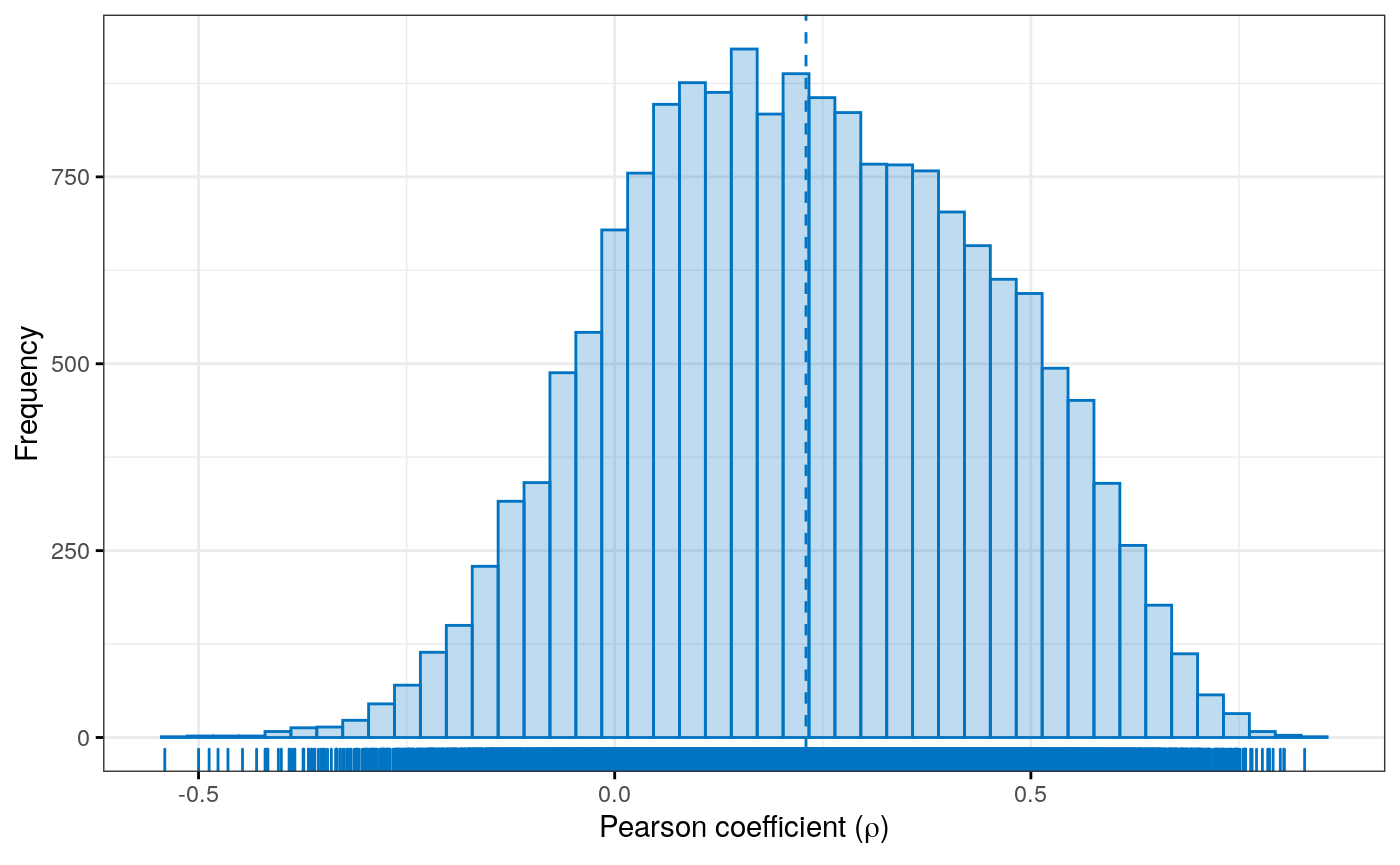
Figure 5
Histogram of the distribution of Pearson correlation coefficients between gene copy number and RNA-seq gene expression in adrenocortical carcinoma (ACC)
Histogram of the distribution of Pearson correlation coefficients between RNA-Seq and copy number alteration in adrenocortical carcinoma (ACC). An integrative representaiton readily allows comparison and correlation of multi-omics experiments.
diagvals <- diag(corres)
diagframe <- data.frame(genename = names(diagvals), value = diagvals)

jco <- get_palette(palette = "jco", 1)

gghistogram(diagframe, x = "value", color = jco, fill = jco, ylab = "Frequency",
    xlab = expression(paste("Pearson coefficient (", rho, ")")), alpha = 0.25,
    ggtheme = theme_bw(), rug = TRUE, bins = 45, add = "mean")
Code for saving as PDF:
# png("F5_rnaseq-cn-correl_ggpubr.png", width = 8, height = 6, units = "in",
#    res = 300)
pdf("F5_rnaseq-cn-correl_ggpubr.pdf", width = 8, height = 6, paper = "special")

gghistogram(diagframe, x = "value", color = jco, fill = jco, ylab = "Frequency",
    xlab = expression(paste("Pearson coefficient (", rho, ")")), alpha = 0.25,
    ggtheme = theme_bw(), rug = TRUE, bins = 45, add = "mean")

dev.off()
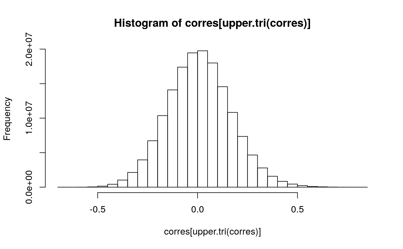
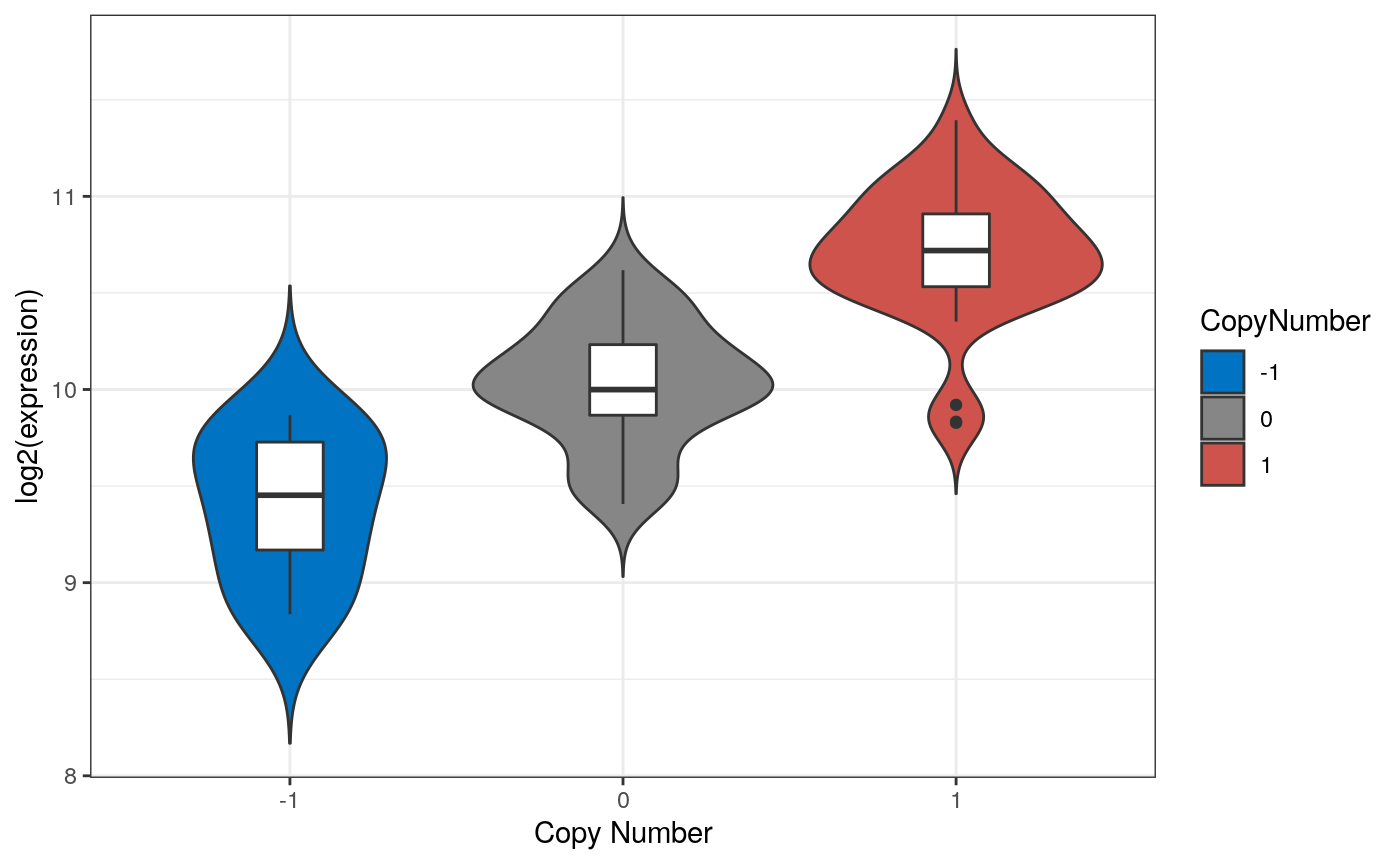
Figure 6
Violin plots
Log 2 expression values by copy number alteration for the highly correlated SNRPB2 gene in adrenocortical carcinoma tumors. Violin plots show differences in expression by copy number loss or gain of SNRPB2, the gene with the highest corration of expression to copy number values (0.83). Copy number increases as log 2 expression values also increase.
##    SNRPB2     NAA20    CRNKL1      BAG5    POLR2C     UBOX5
## 0.8289331 0.8046060 0.8038552 0.7997314 0.7910225 0.7866916
The ‘SNRPB2’ gene expression has a correlation to CNV = 0.83
snr <- subacc[names(topvals)[1L], ]
snpexp <- as.data.frame(wideFormat(snr, check.names = FALSE))
names(snpexp) <- c("primary", "CopyNumber", "Expression")
## remove outlier in CN
table(snpexp$CopyNumber)
##
## -2 -1  0  1
##  1  9 29 38
snpexp <- snpexp[snpexp$CopyNumber != -2, ] snpexp[["Log2Exp"]] <- log(snpexp[["Expression"]], 2) snpexp$CopyNumber <- factor(snpexp$CopyNumber) jcols <- get_palette(palette = "jco", 4) jcols <- jcols[c(1, 3, 4)] ggplot(snpexp, aes(CopyNumber, Log2Exp, fill = CopyNumber)) + geom_violin(trim = FALSE) + xlab("Copy Number") + ylab("log2(expression)") + geom_boxplot(width=0.2, fill = "white") + scale_fill_manual(values = jcols) + theme_bw()
Code for saving as PDF:
# png("violin_exp.png", width = 8, height = 6, units = "in", res = 300)
pdf("F6_violin_exp.pdf", width = 8, height = 6, paper = "special")

ggplot(snpexp, aes(CopyNumber, Log2Exp, fill = CopyNumber)) +
    geom_violin(trim = FALSE) +
    xlab("Copy Number") +
    ylab("log2(expression)") +
    geom_boxplot(width=0.2, fill = "white") +
    scale_fill_manual(values = jcols) +
    theme_bw()

dev.off()
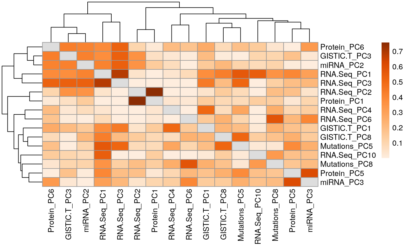
Supplemental Figure 4
Identifying correlated principal components
Correlated Principal Components across experimental assays in Adrenocortical carcinoma (ACC) from The Cancer Genome Atlas (TCGA). Plot identifies correlated principal components across protein, GISTIC copy number, microRNA, mutation, and RNA-Seq assays obtained from curatedTCGAData. The RNA-Seq PC is consistently correlated with protein arrays, GISTIC, and miRNA.
Perform Principal Components Analysis of each of the five assays, using samples available on each assay, log-transforming RNA-seq data first. Using the first 10 components, calculate Pearson correlation between all scores and plot these correlations as a heatmap to identify correlated components across assays.
acc_full <- curatedTCGAData("ACC",
    assays = c("RNASeq2*", "GISTIC_T*", "RPPA*", "Mutation", "miRNASeqGene"),
    dry.run = FALSE)
acc_full
## A MultiAssayExperiment object of 5 listed
##  experiments with user-defined names and respective classes.
##  Containing an ExperimentList class object of length 5:
##  [1] ACC_GISTIC_ThresholdedByGene-20160128: SummarizedExperiment with 24776 rows and 90 columns
##  [2] ACC_miRNASeqGene-20160128: SummarizedExperiment with 1046 rows and 80 columns
##  [3] ACC_Mutation-20160128: RaggedExperiment with 20166 rows and 90 columns
##  [4] ACC_RNASeq2GeneNorm-20160128: SummarizedExperiment with 20501 rows and 79 columns
##  [5] ACC_RPPAArray-20160128: SummarizedExperiment with 192 rows and 46 columns
## Features:
##  experiments() - obtain the ExperimentList instance
##  colData() - the primary/phenotype DataFrame
##  sampleMap() - the sample availability DFrame
##  `$`, `[`, `[[` - extract colData columns, subset, or experiment
##  *Format() - convert into a long or wide DataFrame
##  assays() - convert ExperimentList to a SimpleList of matrices
getLoadings <- function(x, ncomp=10, dolog=FALSE, center=TRUE, scale.=TRUE) { if (dolog){ x <- log2(x + 1) } pc <- prcomp(x, center=center, scale.=scale.) t(pc$rotation[, 1:10]) }
Take only samples that match accross assays:
acc2 <- intersectColumns(acc_full)
Categorize by silent mutations:
mut <- assay(acc2[["ACC_Mutation-20160128"]], i = "Variant_Classification")
mut <- ifelse(is.na(mut) | mut == "Silent", 0, 1)
acc2[["ACC_Mutation-20160128"]] <- mut
Add loadings as a separate assay for each:
acc2 <- c(acc2,
    `RNA-Seq` = getLoadings(assays(acc2)[["ACC_RNASeq2GeneNorm-20160128"]],
        dolog=TRUE), mapFrom=1L
    )
acc2 <- c(acc2,
    `GISTIC-T` = getLoadings(assays(acc2)[["ACC_GISTIC_ThresholdedByGene-20160128"]],
        center=FALSE, scale.=FALSE), mapFrom=2L)
acc2 <- c(acc2,
    Protein = getLoadings(assays(acc2)[["ACC_RPPAArray-20160128"]]),
        mapFrom=3L)
acc2 <- c(acc2,
    Mutations = getLoadings(assays(acc2)[["ACC_Mutation-20160128"]],
        center=FALSE, scale.=FALSE), mapFrom=4L)
acc2 <- c(acc2,
    miRNA = getLoadings(assays(acc2)[["ACC_miRNASeqGene-20160128"]]),
        mapFrom=5L)
Now subset to keep only the PCA results:
acc2 <- acc2[, , 6:10]
## harmonizing input:
## removing 215 sampleMap rows not in names(experiments)experiments(acc2)
## ExperimentList class object of length 5:
##  [1] RNA-Seq: matrix with 10 rows and 43 columns
##  [2] GISTIC-T: matrix with 10 rows and 43 columns
##  [3] Protein: matrix with 10 rows and 43 columns
##  [4] Mutations: matrix with 10 rows and 43 columns
##  [5] miRNA: matrix with 10 rows and 43 columns
Note, it would be equally easy (and maybe better) to do PCA on all samples available for each assay, then do intersectColumns at this point instead.
Now, steps for calculating the correlations and plotting a heatmap: * Use wideFormat to paste these together, which has the nice property of adding assay names to the column names. * The first column always contains the sample identifier, so remove it. * Coerce to a matrix * Calculate the correlations, and take the absolute value (since signs of principal components are arbitrary) * Set the diagonals to NA (each variable has a correlation of 1 to itself).
df <- wideFormat(acc2)[, -1]
mycors <- cor(as.matrix(df))
mycors <- abs(mycors)
diag(mycors) <- NA
To simplify the heatmap, show only components that have at least one correlation greater than 0.5.
has.high.cor <- apply(mycors, 2, max, na.rm=TRUE) > 0.5
mycors <- mycors[has.high.cor, has.high.cor]

# colors
mycolors <- colorRampPalette(brewer.pal(n = 7, name = "Oranges"))(100)
pheatmap::pheatmap(mycors, color = mycolors, angle_col = 90)